3 语法分析 | Parsing¶

约 6918 个字 69 行代码预计阅读时间 24 分钟

朋辈辅学录播

编译原理速成(1) 词法分析&语法分析(上)

编译原理速成(2) 语法分析(中) CFG与自顶向下分析

编译原理速成(3) 语法分析(下) LL(1)与自底向上分析

此部分介绍 语法分析 (Parsing) 和 上下文无关文法 (Context-Free Grammar, CFG) 的相关概念以及 自顶向下分析 (Top-Down Parsing) 的有关内容。

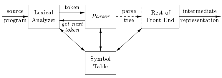
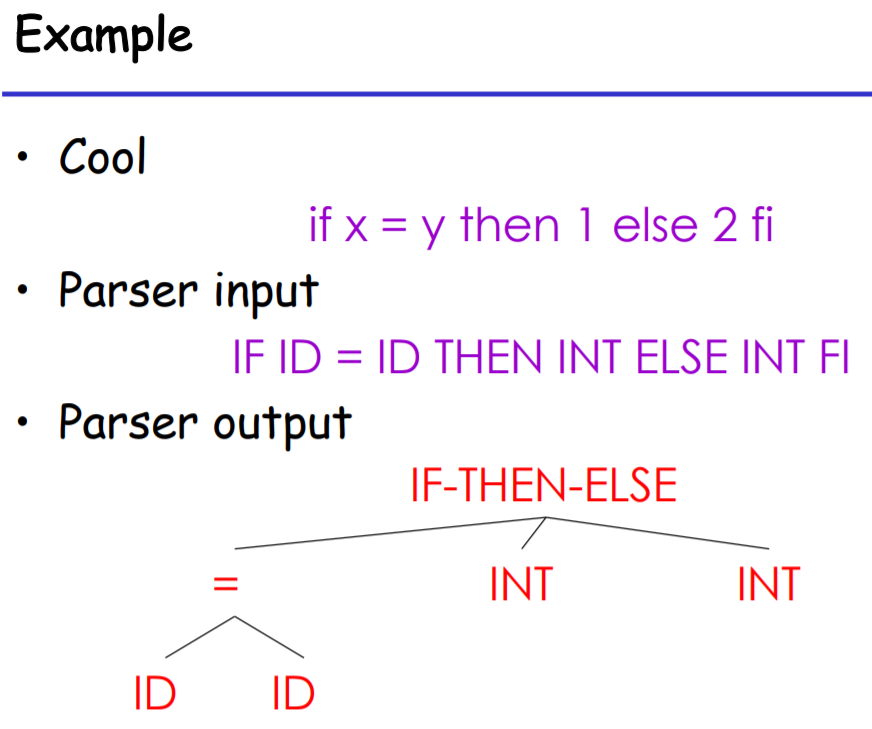
输入：词法分析生成的 token 流；输出：语法分析树/中间表示

Input: sequence of tokens from lexer; Output: parse tree of the program (But some parsers never produce a parse tree ...)

在 2.5 节给出的 Lex 示例中，我们用名字 digits 作为了数字 [0-9]+ 的别名。这种别名使得我们使用 Lex 编写词法规范时更加容易理解。实际上，这种别名的实现非常简单：Lex 在利用正则表达式生成有限自动机之前，用 [0-9]+ 代替 digits 的所有出现即可。这与 C 语言中的宏定义类似。

但是，正如我们在习题 2.2 中探讨过的那样，正则表达式不能实现对括号等的嵌套识别。考虑下面的定义：

digits = [0-9]+
sum     = expr "+" expr
expr    = "(" sum ")" | digits

那么，形如 19 ， 5+6 ， ((1+2)+(3+4)) 等的表达式都可以被上述规则包括（分别对应 digits, sum 和 expr）。其中所有括号都是配对的，但是有限自动机无法实现这种配对的识别。因此，sum 和 expr 不可能被正则表达式表示。这种递归而获得的额外的表示能力正是语法分析所需要的。

3.1 上下文无关文法 | Context-Free Grammars, CFGs¶

如我们所说，编程语言具有递归结构。如同我们用正则表达式静态地定义词法结构一样，我们使用 上下文无关文法 静态地定义语法结构。我们在稍后讨论“上下文无关”的含义。

一个 CFG 描述一种语言。它包括：

A set of terminals $T$
A set of non-terminal $N$
A start symbol $S (\in N)$
A set of productions $X \to y_1y_2...y_n$ , where $X\in N$, $y_1y_2...y_n\in T\cup N\cup \{\epsilon\}$

其中 production 集合是 CFG 描述语言的形式， $X \to y_1y_2...y_n$ 表示 $X$ 可以被 $y_1y_2...y_n$ 替换。Terminal 集合 T 中的符号是该语言字母表中的 tokens，其意义是确定的。Non-terminal 集合 N 中的符号出现在某个 production 的左侧，即它的意义并未确定，还可以进行迭代。

CFG 描述的语言从 start symbol S 出发，将字符串中任何 non-terminal 用某个 production 右侧的东西替换，不断重复直到字符串中没有 non-terminal。亦即，一个 CFG 描述的语言即为自 start symbol 开始，经有限个 production 推导可以得到的 terminal 串的集合。

例如：

EXPR -> if EXPR then EXPR else EXPR fi
      | while EXPR loop EXPR pool
      | id

这里的“|”是或。一般我们将 non-terminal 用大写表示，将 terminal 用小写表示，将 start symbol 写在第一个表达式的左侧。上例等同于：

EXPR -> if EXPR then EXPR else EXPR fi
EXPR -> while EXPR loop EXPR pool
EXPR -> id

也就是说，我们在 CFG 中可以不适用可选符号 | 和克林闭包 *，即：

aux -> c|d 可写为 aux -> c , aux -> d
expr -> aux* 可写为 expr -> aux expr，expr -> ϵ

举一个更加详细的例子。看下面一个 CFG （文法 3-1）：

S -> S; S
S -> id := E
S -> print(L)

E -> id
E -> num
E -> E + E
E -> (S, E)

L -> E
L -> L, E

这个文法有 S E L 三个 non-terminal，有 terminal ; id := print ( ) num + , ，与它对应的源程序可以是 a := 7; b := c + (d := 5 + 6, d); print(b) ，这个源程序经词法分析后是 id := num; id := id + (id := num + num, id); print(id) 。

3.1.1 推导 | Derivation¶

如果存在 production A -> a ，那么串 xay 就是表达式 xAy 的一个实例，我们称 xAy => xay ，即 xAy经过一步推导出 xay 。在 => 上增加 * 或 + 表示经过零或多步、一或多步推导出。推导证明一个句子属于一个 CFG 的语言。

例如文法 3-1 的一个句子 a := 7; b := c + 2 可以经如下推导：

S
S; S
id := E; S
id := num; S
id := num; id := E
id := num; id := E + E
id := num; id := id + E
id := num; id := id + num

在上面的推导中，我们每一次选取最左边的非终结符进行扩展，因此称为 最左推导 (leftmost derivation) ，类似地，也有 最右推导 (rightmost derivation) 。当然，推导也可以既不是最左推导，也不是最右推导。

但是，如 a := 1; b := 2; c := 3 的句子有两种不同的 最左推导 ：

- `S` => `S; S` => `id := num; S` => `id := num; S; S` =>...
- `S` => `S; S` => `S; S; S` => `id:= num; S; S` =>...

这种现象说明文法是 二义性的 (ambiguous) ，我们将在 3.1.3 小节讨论这个问题。

3.1.2 语法分析树 | Parse Tree¶

推导过程中，我们对每个非终结符进行扩展。将非终结符作为父结点，扩展出的内容作为子结点，则可以形成一棵树，即语法分析树。3.1.1 例子的语法分析树为：

可以看到，语法分析树的所有叶子结点均为 terminals，其他节点均为 non-terminals。叶子结点的中序遍历即为原输入。与原输入相比，语法分析树显示了 token 之间的联系。每种推导对应了一棵语法分析树，但是每棵语法分析树可以对应多种推导方式。

可以说明，对于每一种最左推导，一定有且仅有一种最右推导与其形成同样的语法分析树；其区别只是树的分支加入的顺序。

3.1.3 二义性 | Ambiguity¶

看下面一个例子：

Grammar: E -> E+E | E*E | (E) | id

String: id * id + id

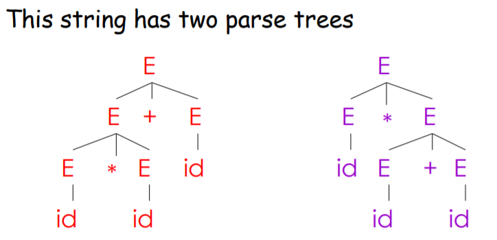
这两棵语法分析树分别对应两种最左推导：

E => E+E => E*E+E => ...
E => E*E => E*E+E => ...

这两种推导方式都是符合文法的最左推导。

如果一个文法会使某些字符串有不止一个语法分析树，即该字符串有多种最左推导（或对应地，有多种最右推导），则称这个文法有二义性。我们希望文法是无二义性的。

需要解决二义性，最直接的方法是重新写一个没有二义性的文法（好呆瓜）。上例中，我们一般选取左边那种理解，因为我们认为 * 比 + 具有更高的 优先级 (precedence) 。那么我们可以通过重写，强制这种优先级：

Grammar : E -> T+E | T , T -> F*T | F , F -> id | (E)

通过这种方式，我们强制了 id 和 () 具有最高优先级（因为他们会被作为一个整体展开），* 次之， + 优先级最低。这样，上例就只有唯一一种最左推导：

E => T+E => F*T+E => ...

即消除了二义性。

我们再考虑这样一个例子：

Grammar : E -> E-E | num ， String : 3-2-1

可以发现，这样一个简单的文法也有两种不同的最左推导，分别得到 (3-2)-1 和 3-(2-1) 两种结果，显然我们希望的是前一种。这个问题的原因是 结合性 (associativity) ，我们希望 - 是左结合的。因此我们可以通过重写，强制这种结合性：

Grammar : E -> E-T , T -> num

这样就消除了二义性。

需要说明的是，这里并没有一种通用的方法来解决二义性（Why？），因此我们只能通过人工的方式完成上面那样的消除二义性文法的重写。但是我们同时可以发现，这种重写会使得文法变得复杂，难以阅读和维护。因此，我们尝试通过某种消除二义性的声明来接受二义性，因为这样的文法更加简单和自然。

大多数工具采取这样的方法。这些工具通过声明 precedence & associativity 来消除文法中的二义性。

The parser doesn't really understand about associativity & precedence. Instead, these declarations tell it to make certain kind of moves in certain situations. We won't be able to explain this until we get much further into parsing technology.

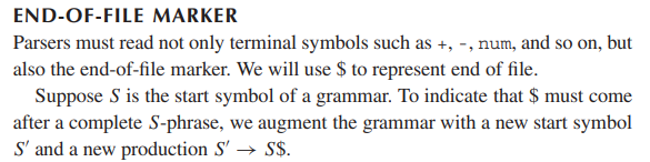
3.1.4 文件结束符 | EOF Marker¶

3.1.5 上下文无关 | Context Free¶

我们所说的“上下文无关”或者“静态”，这里解释的很清楚（其实就是字面意思）：

那么什么是上下文有关呢？我们可以说，如果只有对特定的串 β 和 γ，才有规则 βAγ -> βαγ 时，我们称这条规则是上下文有关的。实际上，我们在 C 语言中需要先声明后使用就是一种上下文有关的例子。即：

{
     int x;
     ...
     ...x...
     ...
}

如果给相关的规则加上一些限制，那么我们有可能可以使用 BNF 来完成对上述上下文有关文法的分析；但即使如此，这个工作量是巨大的。因此，我们将这些信息和限制放到稍后去处理。在语法分析部分，我们暂时只考虑上下文无关文法的分析。

3.2 递归下降分析 | Recursive Descent Parsing¶

Recursive Descent Parsing 是 自顶向下分析 (Top-Down Parsing) 的一种。所谓 Top-Down Parsing，就是从顶（start symbol）开始，从上到下、从左到右构造 parse tree。

3.2.1 思路¶

递归下降利用的核心思路是，parse tree 叶子结点的中序遍历即为输入的 token 流。

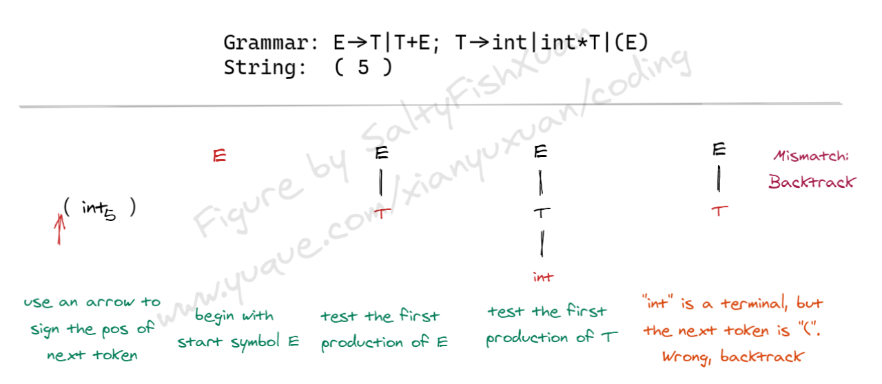
递归下降分析的过程，即从上到下、从左到右，对 parse tree 中的每一个结点进行遍历。对于遍历到的每个结点，如果该点是

Terminal，则查看下一位输入是否与该 terminal 相同。如果相同，则接受该输入；如果不同，或者没有下一位输入，则说明出现了错误，进行 backtrack，即回溯到上一步 non-terminal（因为 terminal 一定由 non-terminal 引出）；
Non-terminal，则：
- 尝试第一个从该 non-terminal 引出的 production，即将该 production 的右端作为该结点的子结点加入 parse tree，然后依次遍历子结点
- 如果 backtrack 到了当前 non-terminal，则尝试下一个 production
- 如果 backtrack 到了当前 non-terminal 但所有 production 都已经尝试完了，那么说明该 non-terminal 是不应当出现的，回溯到上一步 non-terminal。

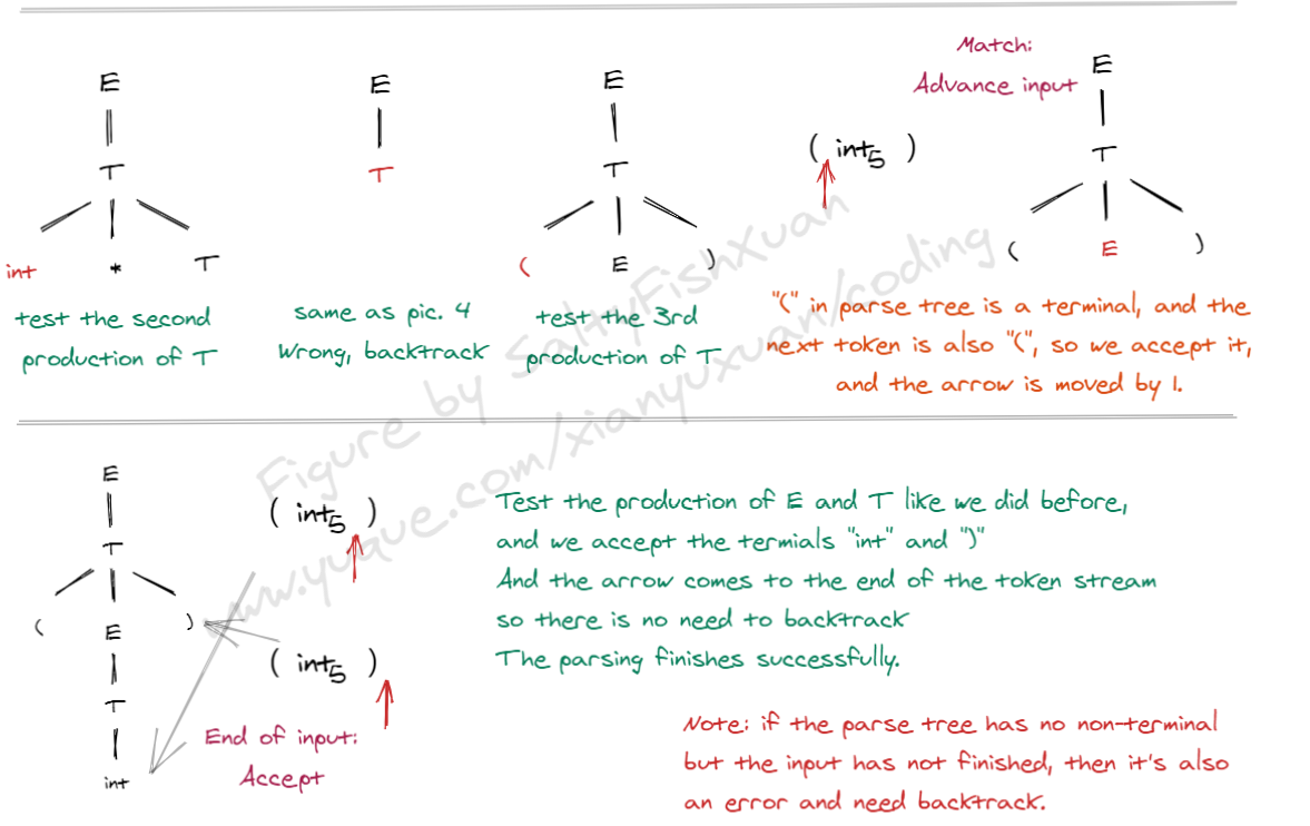
重复该步骤，直到所有结点都被遍历完。如果此时输入已经结束，那么我们找到了一个匹配的 parsing；否则说明仍然存在错误，继续 backtrack。

下面是递归下降分析的一个实例：

3.2.2 实现¶

Grammar: E -> T | T+E, T -> int | int * T | (E)

我们用 C 语言尝试实现 Recursive Descent Parser：

我们用 TOKEN 表示 token 的类型，用指针 next 指向下一个 token（Line 1~4）
我们用一系列函数进行前述思路中的检查和尝试，这些函数的返回值类型为 bool ，用来表示识别成功与否。如果不成功，我们进行回溯。这里的 parse tree 实际上是由函数的嵌套关系组织的，因此所谓“回溯”除了函数的自然返回，就只需要将 next 回到之前的位置即可。
- bool term(TOKEN tok) 是对 terminal 的检查，顺便把 next++
- bool E1() 是 non-terminal E 的第一个 production E -> T 。可以看到其返回 true 的条件即为 T() 为真。类似地， bool E2() 是 production E -> T+E 对应的函数，返回 true 的条件为依次匹配到 T() , term(PLUS) （即 terminal "+"）和 E() 。
- bool E() 是 non-terminal E 的所有 production 的集合，注意到 11 行首先保存 next 到 save ，用来回溯；然后 12 行首先判断 E1() 是否为真：
  - 如果为真则根据 C 语言的短路规则，其后的 (next = save, E2()) 并不会被运行，直接返回真；
  - 如果不为真则运行 (next = save, E2()) ，即首先恢复 next ，然后判断 E2() 是否为真。
    需要特殊说明的是，这里第 12 行的 (next = save, E1()) 中的 next = save 并没有作用，因为第 10 行刚刚将 save 赋值为 next ，这里只是为了整齐，去掉也可以。
- 开始 parsing 时，我们只需要调用 start symbol 对应的函数，即 E() 。

enum TOKEN {INT, OPEN, CLOSE, PLUS, TIMES};
          /* int    (        )        +      -    */
TOKEN input[MAXN];
TOKEN *next = input;

bool term(TOKEN tok) { return *next++ == tok; }

bool E1() { return T(); }
bool E2() { return T() && term(PLUS) && E(); }
bool E() {
     TOKEN *save = next; 
     return (next = save, E1()) 
          || (next = save, E2()); 
}

bool T1() { return term(INT); }
bool T2() { return term(INT) && term(TIMES) && T(); }
bool T3() { return term(OPEN) && E() && term(CLOSE); }
bool T() { 
     TOKEN *save = next; 
     return (next = save, T1())
        || (next = save, T2())
        || (next = save, T3()); 
}

但是，我们考虑这样一种情况： S -> Sa

则我们会写出这样两个函数： bool S1() { return S() && term(a); } , bool S() { return S1(); } ，我们可以发现 S() 进入了死循环。这种情况称为 左递归 (left-recursive) 。

3.2.3 左递归 | Left-Recursive¶

承上例，如果存在一个 non-terminal S 使得 S ->+ Sa ，即经过 1 个或多个 production 后，S 可以产生一个由 S 开头的右端，那么我们用前述方法生成的 Recursive Descent 代码就不能够完成语法分析，因为它会陷入死循环。这是左递归的一般形式。

实际上，左递归可以被机械地（即，有一般方法地）消除。考虑这样一种文法： S -> Sa | b ，实际上这种文法生成的是一个 b 以及若干个 a 。我们可以将它重写为 右递归 (right-recursion) 的形式： S -> bT , T -> aT | ϵ。这两种文法的区别是，我们将递归移到了产生式的最右边，而这是可以被 Recursive Descent 接受的形式。

实际上，我们实现 Recursive Descent Parsing 时，在 3.2.2 小节中展示的步骤之前，我们需要首先将文法改写成没有左递归的形式。

3.2.4 总结¶

Recursive Descent 是一种非常简单而且通用的方法，因为其过程比较简单，且虽然左递归需要提前消除，但是消除左递归的过程是比较简单的，而且可用算法自动完成。在实际操作中，人们通常手动将左递归消除，因为编译器的设计者需要知道 parser 使用何种文法，且消除左递归是容易的。

由于 Recursive Descent 需要 backtrack，在过去被人们认为非常低效，因此不很常用；在如今的机器上 Recursive Descent 是非常快速和简单的，因此在如今非常流行。例如 gcc 就用到了手写的 Recursive Descent。

3.3 LL(1) Parsing¶

预测分析 (Predictive Parsing) 也是一种 Top-Down Parsing，它通过查看当前输入位置之后的几个 token 来决定使用哪一个 production，从而避免了 backtracking。

预测分析器可以用于处理 LL(k) 文法，LL(k) 各部分的含义是：

第一个 L：left-to-right scan of input
第二个 L：leftmost derivation
k：predict based on k tokens of lookahead

我们这里讨论 LL(1) 文法，即通过查看当前 token 之后的一个 token 就能决定使用哪个 production 的文法。

3.3.1 思路¶

对于 Recursive Descent，每一步有多种可选的 production；Backtracking used to undo bad choices.

对于 LL(1)，每一步只会有一个或零个 (error state) 可以选择的 production。由于 "LL"，因此实际上我们每次只需要将最左端的 non-terminal 用一个 production 的右端替换；而 "(1)" 要求我们只查看输入中的 1 个 token 就可以知道使用哪一个 production；即：每一个 production 右端的第一个 terminal 是唯一的。在这样的条件下，我们可以通过不断的展开和查看 production 来完成 token 流的语法分析。

这一要求对大多数文法来说是不能满足的，但是我们可以通过一些方法来满足这一要求。

3.3.2 提取左因子 | Left Factoring¶

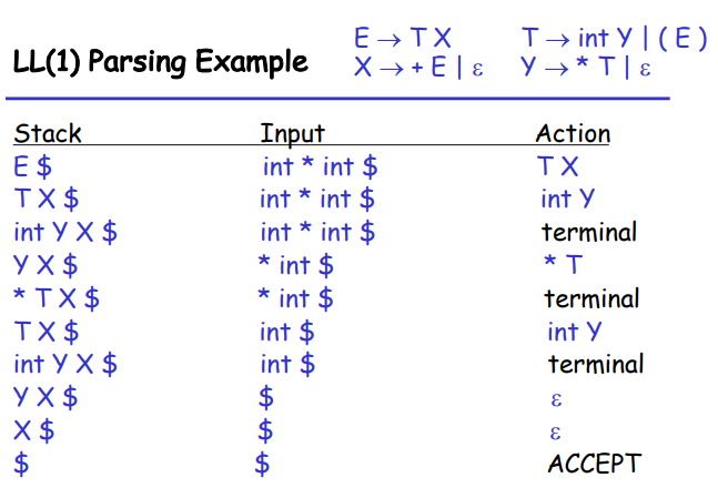
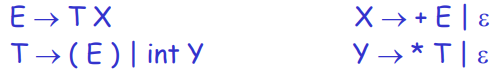
我们仍然讨论 3.2 中用到的文法： E -> T+E | T , T -> int | int*T | (E)

3.3.3 预测分析表 | Predictive Parsing Table¶

如我们之前所说，我们需要根据每一个当前最左端的 non-terminal 以及 lookahead 得到的 next input token 来选取唯一的 production。因此我们可以通过一个表格来表示这种预测关系，下图是上述文法的对应例子（我们稍后再讨论这张表的建立方式）：

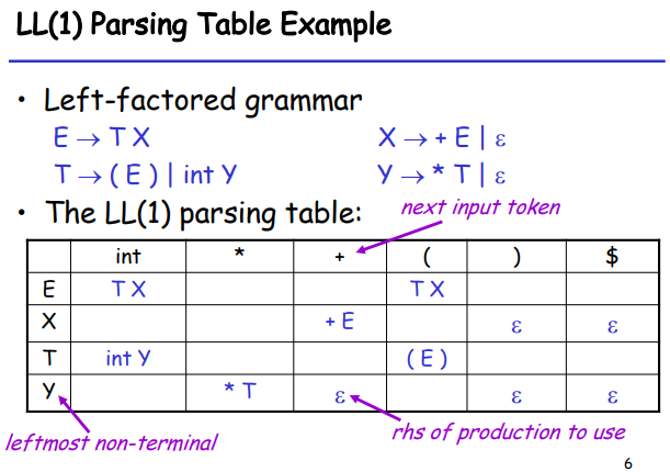
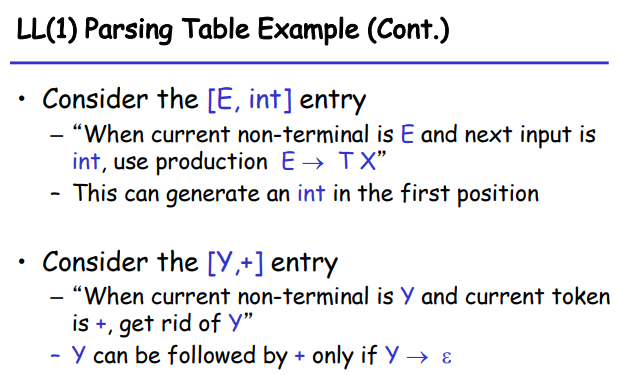
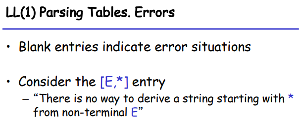
本文中，如果 Parsing Table 中 non-terminal A 和 terminal t 对应的项目为 a ，那么记 T[A,t] = a 。

3.3.4 使用预测分析表¶

由于我们的语法分析过程始终只需要考虑最左端的 non-terminal，我们可以用一个栈来存储正在生成的 parse tree，栈顶即为 leftmost non-terminal 或者即将被匹配的 leftmost terminal（如果与输入相同则出栈，如果不同则说明出现了语法错误）。如果出现了 error state，则也说明出现了语法错误；如果栈为空且输入结束，则语法分析成功结束。

下面是 LL(1) Parsing 的算法：

initialize stack = {S, $}
repeat
    case stack.top of
     X: //non-terminal
            if T[X, *next] = Y1...Yn then
                pop X
                push Y1...Yn onto stack
          else
                error()
     t: //terminal
            if t == *next++ then
                pop t
          else
                error()
until stack == {}

其中：

Line 1, 14：S 是 Start Symbol，$ 是输入的末尾，如果最终 stack 为空，说明栈为空（除了 $）的同时输入到达结束，即 parsing 被接受。
Line 3：当栈非空时，我们不断进行这一工作：检查栈顶是 non-terminal 还是 terminal，如果：
- 为 non-terminal，那么根据该 non-terminal（即 leftmost）以及输入的下一个 token（即 *next ）在 Parsing Table 中进行查找，如果该项为空说明出现错误（Line 7~8）；否则将表中的对应内容，即 T[X, *next] 压入栈顶，即栈从 {X, rest} 变为 {Y1, ..., Yn, rest} 。Production 右端的 leftmost symbol 成为新的栈顶。
- 为 terminal，这种情况与之前的 Recursive Descent 中对 terminal 的处理一致。

下面是一个例子：

3.3.5 构造预测分析表¶

对于 non-terminal A , production A->X , token t , 则 T[A, t] = X 当且仅当：

X ->* tY ，即 X 可以经 0 步或多步转换成一个由 t 开头的串。这时我们记 $t\in\text{First}(X)$。或者
X ->* ϵ 且 S ->* pAtq ，其中 p 和 q 为任意串（可为空）；即存在从 Start Symbol 开始的任一步推导包含 At ，且 X 可为空。这时我们记 $t\in \text{Follow}(X)$。

上面所述的 $\text{First}(X)$ 和 $\text{Follow}(X)$ 是 terminal 的两个集合。我们给出这两个集合的定义和解释：

3.3.5.1 First Sets¶

给定符号 X ，$\text{First}(X)$ 表示可以从 X 中推导出的所有 terminal 串中 leftmost terminal 的集合。这里给出一个形式化的定义：

$\text{First}(X) = \{t\ |\ X\Rightarrow^* t\alpha\} \cup\{\epsilon\ |\ X\Rightarrow^* \epsilon\}$ 即，如果 X 可以经 0 步或多步推导出以 terminal t 开头的串，那么 t 属于 $\text{First}(X)$（$\alpha$ 是什么并不重要，它只是用来表示 t 后面还可以有东西）；如果 X 可以经 0 步或者多步推导出空串，那么 ϵ 属于 $\text{First}(X)$。

我们可以按照如下思路计算出 First Sets：

举个例子，我们仍然研究刚刚的文法：

首先， X , Y , T 的 First 集合是显然的，因为它们的每一种产生式的开头都是 terminal：

$\text{First}(X) = \{+,\epsilon\},\quad \text{First}(Y) = \{*,\epsilon\},\quad \text{First}(T) = \{\ (\ ,\text{int}\}$

另外注意 E -> TX ，有 $\text{First}(T)\subseteq \text{First}(E)$；进一步我们发现 T 不可能导出空串，因此 $\text{First}(E)$ 没有其他元素了。因此 $\text{First}(E) = \{\ (\ ,\text{int}\}$。

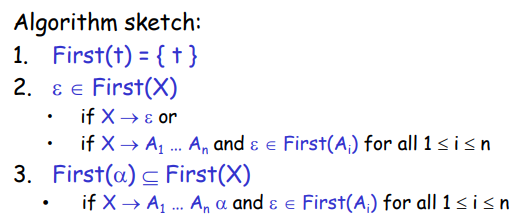
一般地，对于一个非终结符 X ，计算它的 First 集合的算法是：（Ref：Link）

/* 遍历所有 production。即，在以这个 Non-terminal 为左端的一个 production 中：*/

// If epsilon not found in the first set of the current token or
// the current token is the last one in the production, then add all
// the tokens to the first set and don't continue evaluating the next tokens
// Example 1:
//        A -> B C D
//        B -> 'T1' | 'T2'
//        ...
// Then First(A) contains First(B)
// Example 2:
//        A -> B C D
//        B -> EPSILON | 'T1'
//        C -> 'T2' | 'T3'
//        ...
// Then First(A) contains First(B)-{EPSILON} U First(C)
// Example 3:
//        A -> B C D
//        B -> EPSILON | 'T1'
//        C -> EPSILON | 'T2'
//        D -> EPSILON | 'T3'
//        ...
// Then First(A) contains First(B)-{EPSILON} U First(C)-{EPSILON} U First(D).
// Note that in Example 3, EPSILON will be in First(A)

我们遍历每一条 production。对于每一条 production，记左边的 non-terminal 为 X，我们遍历其右边的 tokens：

如果是$\epsilon$或者 terminal，将其加入 X 的 First Set 并且停止遍历。因为$\epsilon$只会单独出现，而 terminal 后面的东西也不会出现在 X 的 First Set 中了；
如果是 Non-terminal：
- 如果 Non-terminal 的 First Set 中没有$\epsilon$，或者这是当前 production 的最后一个 token，将 Non-terminal 的 First Set 加入 X 的 First Set，然后停止；
- 如果 Non-terminal 的 First Set 中有$\epsilon$，而且不是当前 production 的最后一个 token，将 Non-terminal 的 First Set 中除了$\epsilon$以外的元素加入 X 的 First Set，然后继续遍历。

我们重复对 production 的遍历足够多次（production 的条数次；或者直到一次遍历中所有 First Set 没有发生改变），这样保证每个 First Set 都基于正确的其他 First Set 进行合并。这样就得到了所有 Non-terminal 的 First Set。

3.3.5.2 Follow Sets¶

给定符号 X ，$\text{Follow}(X)$ 表示可以从 Start Symbol S 推导出的所有串中，可能直接接在 X 之后的 terminal 的集合。我们同样给出一个形式化的定义：

$\text{Follow}(X) = \{t\ |\ S\Rightarrow^*\alpha Xt\beta\}$ 同样的，这里 $\alpha, \beta$ 是什么也并不重要，它只是用来表示 Xt 的前后还可以有东西。需要注意的是，epsilon 不可能出现在 Follow Sets 中。如果表示当前 token 之后可能什么都没有（即文件结束），则其 Follow Set 包含文件结束符 $ 。因此，Start Symbol S 的 Follow Set 包含文件结束符 $。

一般地，对于一个非终结符 X ，计算它的 Follow 集合的算法是：（Ref：Link）

/* 遍历所有 production 右边的每一个 token。即，对于每个 production 中出现的每个 token： */

// If the current token is a non-terminal then iterate on the next token
// and add its first set to the follow set of the current token except for
// the epsilon value. If the first set had an epsilon value, then the next token
// needs to be evaluated as well. This repeats until no epsilon is found or if
// there are no more tokens in the production, which in that case the follow set
// of the LHS is added to the follow set of the current token.
// Example 1
//        A -> B C D
//        Follow(A) = {'T1'}
//        First(C) = {'T2', EPSILON}
//        First(D) = {'T3'}
// Then Follow(B) contains First(C)-{EPSILON} U First(D)
// Example 2
//        A -> B C D
//        Follow(A) = {'T1'}
//        First(C) = {'T2', EPSILON}
//        First(D) = {'T3', EPSILON}
// Then Follow(B) contains First(C)-{EPSILON} U First(D)-{EPSILON} U Follow(A)

对 Follow Set 的计算是在建立在完成对 First Sets 计算的基础上的。对于每一个 production 右侧的每一个 token X，遍历其后面的 token Ri：将 Ri 的 First Set（减去$\epsilon$）加入 X 的 Follow Set；如果 Ri 的 First Set 不包含$\epsilon$则停止，否则继续遍历下一个 token；如果所有 token 都可以取$\epsilon$，则将 production 左边的 Non-terminal 的 Follow Set 加入 X 的 Follow Set。

3.3.5.3 Construct Predictive Table¶

根据我们计算出的 First Sets 和 Follow Sets，我们可以通过如下算法构造出该文法的预测分析表：

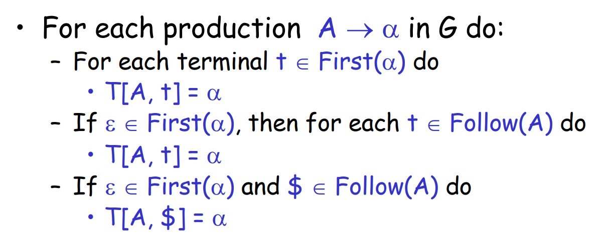
其中， First(α) 是该 production 的右侧的 First Set，其元素其实就是 3.3.5.1 中遍历到对应 production 时加入到 First(A) 的元素。因此，我们可以在 3.3.5.1 中，同时维护一个对于 production 左边 Non-terminal 的 First Set 和这个 production 本身（或者说，它的右边）的 First Set，以便这一步进行使用。

这三条规则的原理是容易理解的，我们逐一解释。

回顾之前对预测分析表的定义，T[A, t] = α 的含义是，如果当前 non-terminal 是 A 且下一个 input token 是 t，那我们采取 A -> α。

第一条规则是说，如果 α 可以以 t 开头，那么 T[A, t] = α。这是显然的，因为当我们采取 A -> α 之后，由于 α 可以以 t 开头，这样就能匹配下一个 input token t 了。

第二条规则是说，如果 α 可以为空，那么对于 Follow(A) 中的每一个 terminal t，T[A, t] = α。这是因为，我们采取 A -> α 之后，可以进一步采取 α => ϵ，这样下一个 terminal 就可能是 Follow(A) 中的任何一个了，因此如果下一个 input token t 在 Follow(A) 中，就可能被匹配。

第三条规则和第二条规则一样，只是单独把 $ 拿出来说一下。所以其实也可以直接记住前面两个规则。

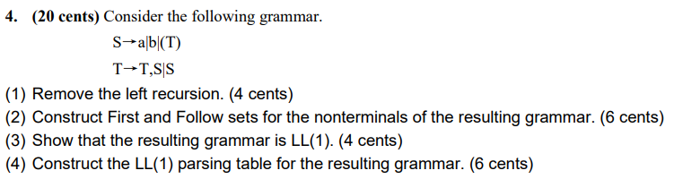
3.3.5.4 例子¶

下面是课本中的一道例题，展示了去除左递归、计算 First 和 Follow Set、构造 LL(1) Parsing Table 和使用 Parsing Table 的过程。

Example

Consider the grammar:

lexp -> atom | list
atom -> number | identifier
list -> (lexp-seq)
lexp-seq -> lexp-seq lexp | lexp

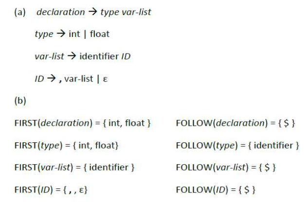
a. Remove the left recursion

b. Construct the First and Follow set of the nonterminals of the resulting grammar.

c. Construct the LL(1) table for the resulting grammar.

d. Show the actions of the corresponding parser, given the following input string (a(b(2))(c)).

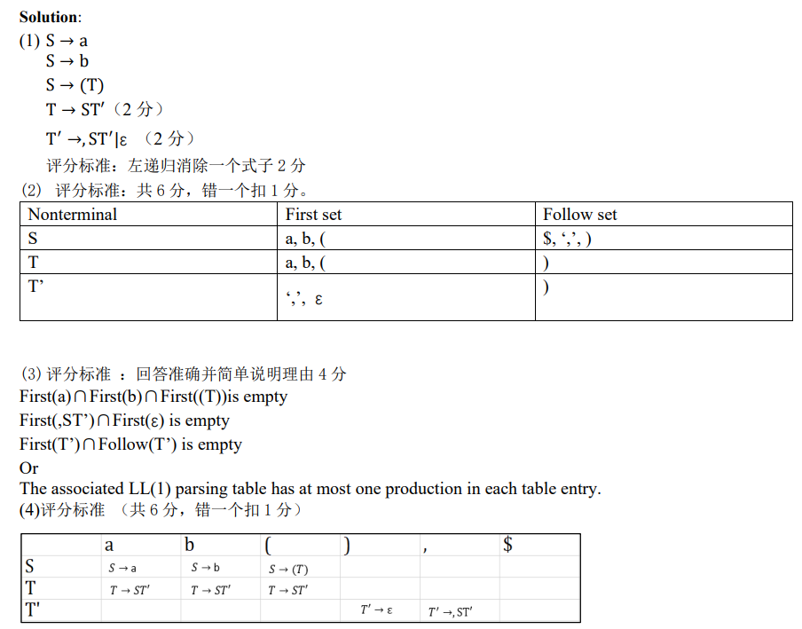
solution

a. Production lexp-seq -> lexp-seq lexp | lexp is left-recursive. We rewrite it to be: lexp-seq -> lexp seq, seq -> lexp seq | EPSILON. That is, the grammar after removing the left recursion is:

lexp -> atom | list
atom -> number | identifier
list -> (lexp-seq)
lexp-seq -> lexp seq
seq -> lexp seq | EPSILON

b.

First Sets:

Terminals: number, identifier, ( and ).

We can first get to know that $First(atom) = \{number,\ identifier\}$ by production 2 and that $First(list) = \{(\}$ by production 3.

From production 1 we know that $First(lexp) = First(atom)\cup First(list) = \{number,\ identifier,\ (\}$, and from production 4 we know that $First(lexp\text-seq) = First(lexp) = \{number,\ identifier,\ (\}$.

From production 5 we know that $First(seq) =First(lexp)\cup \{\epsilon\} = \{number,\ identifier,\ (,\ \epsilon\}$

Follow Sets:

As lexp is the start symbol, there is $\$\in Follow(lexp)$.

From production 1 we can know that $Follow(lexp)\subseteq Follow(atom)$ and $Follow(lexp)\subseteq Follow(list)$.

From production 3 we can know that $\ )\ \in Follow(lexp\text-seq)$

From production 4 we can know that $First(seq) - \{\epsilon\}\subseteq Follow(lexp)$, and as $\epsilon\in First(seq)$, there is also $Follow(lexp\text-seq)\subseteq Follow(lexp)$. It can also be known that $Follow(lexp\text-seq)\subseteq Follow(seq)$ .

Therefore the total first and follow sets are:

Non-terminals	First Sets	Follow Sets
lexp	$\{number,\ identifier,\ (\}$	$\{number,\ identifier,\ (,\ )\ ,\$\}$
atom	$\{number,\ identifier\}$	$\{number,\ identifier,\ (,\ )\ ,\$\}$
list	$\{\ (\ \}$	$\{number,\ identifier,\ (,\ )\ ,\$\}$
lexp-seq	$\{number,\ identifier,\ (\}$	$\{\ )\ \}$
seq	$\{number,\ identifier,\ (,\ \epsilon\}$	$\{\ )\ \}$

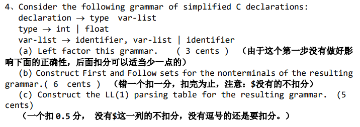
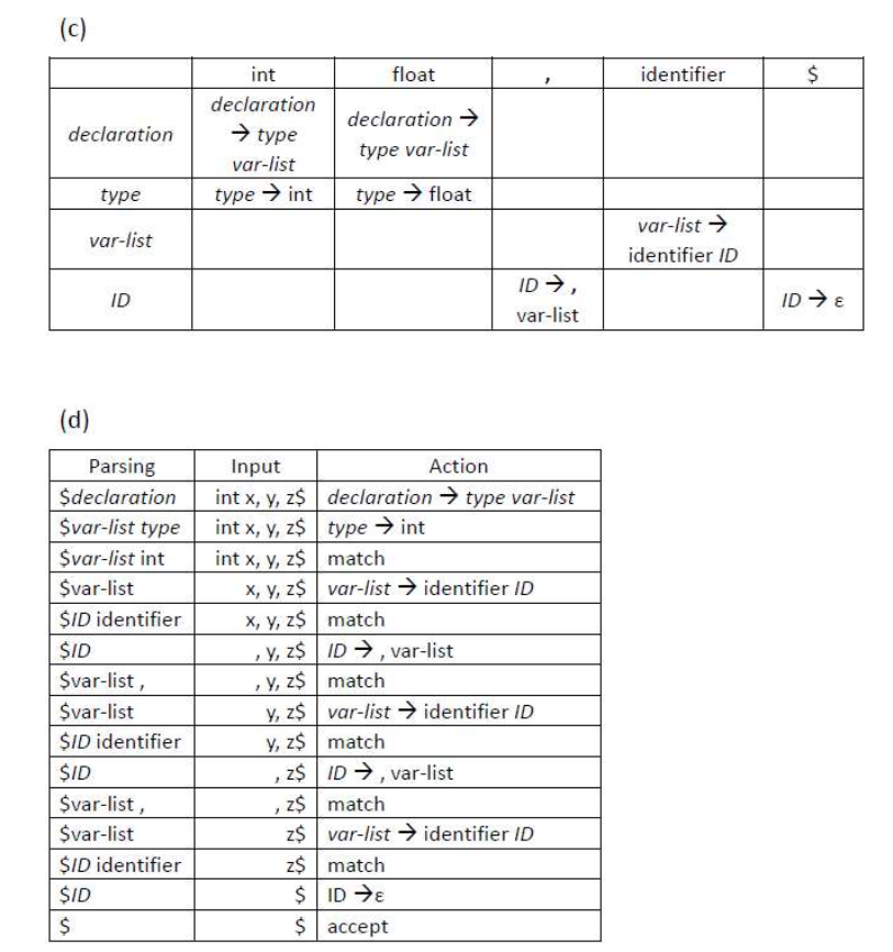
c. We can construct the LL(1) parsing table with the first and follow sets above: (the LHS i.e. Left Hand Side of each production has been omitted as they are shown in the leftmost column of the table)

LHS	number	identifier	(	)
lexp	`->atom`	`->atom`	`->list`
atom	`->number`	`->identifier`
list			`->(lexp-seq)`
lexp-seq	`->lexp seq`	`->lexp seq`	`->lexp seq`
seq	`->lexp seq`	`->lexp seq`	`->lexp seq`	`->EPSILON`

As we can see, there is no conflicting entries in the table, or in other words, there is at most 1 production in each table entry. This satisfies the definition of LL(1) grammar. Therefore the grammar is LL(1).

d.

Stack	Input	Action
lexp $	`(a(b(2))(c))$`	`->list`
list $	`(a(b(2))(c))$`	`->(lexp-seq)`
( lexp-seq ) $	`(a(b(2))(c))$`	Match `(`
lexp-seq ) $	`a(b(2))(c))$`	`->lexp seq`
lexp seq ) $	`a(b(2))(c))$`	`->atom`
atom seq ) $	`a(b(2))(c))$`	`->identifier`
identifier seq ) $	`a(b(2))(c))$`	Match `a`
seq ) $	`(b(2))(c))$`	`->lexp seq`
lexp seq ) $	`(b(2))(c))$`	`->list`
list seq ) $	`(b(2))(c))$`	`->(lexp-seq)`
( lexp-seq ) seq ) $	`(b(2))(c))$`	Match `(`
lexp-seq ) seq ) $	`b(2))(c))$`	`->lexp seq`
lexp seq ) seq ) $	`b(2))(c))$`	`->atom`
atom seq ) seq ) $	`b(2))(c))$`	`->identifier`
identifier seq ) seq ) $	`b(2))(c))$`	Match `b`
seq ) seq ) $	`(2))(c))$`	`->lexp seq`
lexp seq ) seq ) $	`(2))(c))$`	`->list`
list seq ) seq ) $	`(2))(c))$`	`->(lexp-seq)`
( lexp-seq ) seq ) seq ) $	`(2))(c))$`	Match `(`
lexp-seq ) seq ) seq ) $	`2))(c))$`	`->lexp seq`
lexp seq ) seq ) seq ) $	`2))(c))$`	`->atom`
atom seq ) seq ) seq ) $	`2))(c))$`	`->number`
number seq ) seq ) seq ) $	`2))(c))$`	Match `2`
seq ) seq ) seq ) $	`))(c))$`	`->EPSILON`
) seq ) seq ) $	`))(c))$`	Match `)`
seq ) seq ) $	`)(c))$`	`->EPSILON`
) seq ) $	`)(c))$`	Match `)`
seq ) $	`(c))$`	`->lexp seq`
lexp seq ) $	`(c))$`	`->list`
list seq ) $	`(c))$`	`->(lexp-seq)`
( lexp-seq ) seq ) $	`(c))$`	Match `(`
lexp-seq ) seq ) $	`c))$`	`->lexp seq`
lexp seq ) seq ) $	`c))$`	`->atom`
atom seq ) seq ) $	`c))$`	`->identifier`
identifier seq ) seq ) $	`c))$`	Match `c`
seq ) seq ) $	`))$`	`->EPSILON`
) seq ) $	`))$`	Match `)`
seq ) $	`)$`	`->EPSILON`
) $	`)$`	Match `)`
$	`$`	ACCEPT

3.3.6 LL(1) Grammar¶

如果在如上述方法构造出的 LL(1) Parsing Table 中的每一格都至多有 1 个 production，那么对于每一个 current non-terminal 和 next input token 的组合，都有且仅有一种情况（一个 production 或者 error state）与之对应。这样的文法能够利用 LL(1) 完成预测分析，我们称这个文法是 LL(1) 的。

等价地，一个文法是 LL(1) 的，如果：

For every production A→α1|α2|...|αn, First(αi) ∩ First(αj) is empty for all i and j, 1 ≤ i, j ≤ n, i ≠ j.
For every non-terminal A such that First(A) contains EPSILON , First(A) ∩ Follow(A) is empty.

一些相关的问题和参考回答

a. Can an LL(1) grammar be ambiguous? Why or why not? b. Can an ambiguous grammar be LL(1)? Why or why not? c. Must an unambiguous grammar be LL(1)? Why or why not?

参考回答

a. No. For each possible pair of non-terminal on the top of the stack (i.e. leftmost non-terminal) and the input token (i.e. the pending terminal), there is at most 1 production to use. So it's impossible for an input string to get 2+ different parsing trees. So LL(1) grammar must not be ambiguous.

b. No. If the grammar is ambiguous, then there must be some points where 2+ choices are available, which means that there will be 2+ productions in an entry of the parsing table. But this violates the definition of LL(1) grammar. So no ambiguous grammar can be LL(1).

c. No. Left-recursive grammars or grammars without left-factoring may be unambiguous but they are still not LL(1). Other grammars which are complex enough maybe also not LL(1). In fact, most programming language CFGs used now are not LL(1) because of their complexity.

评论区~

有用的话请给我个赞和 star =>

快来跟我聊天~

Non-terminals	First Sets	Follow Sets
lexp	\(\{number,\ identifier,\ (\}\)	\(\{number,\ identifier,\ (,\ )\ ,\$\}\)
atom	\(\{number,\ identifier\}\)	\(\{number,\ identifier,\ (,\ )\ ,\$\}\)
list	\(\{\ (\ \}\)	\(\{number,\ identifier,\ (,\ )\ ,\$\}\)
lexp-seq	\(\{number,\ identifier,\ (\}\)	\(\{\ )\ \}\)
seq	\(\{number,\ identifier,\ (,\ \epsilon\}\)	\(\{\ )\ \}\)